Figures
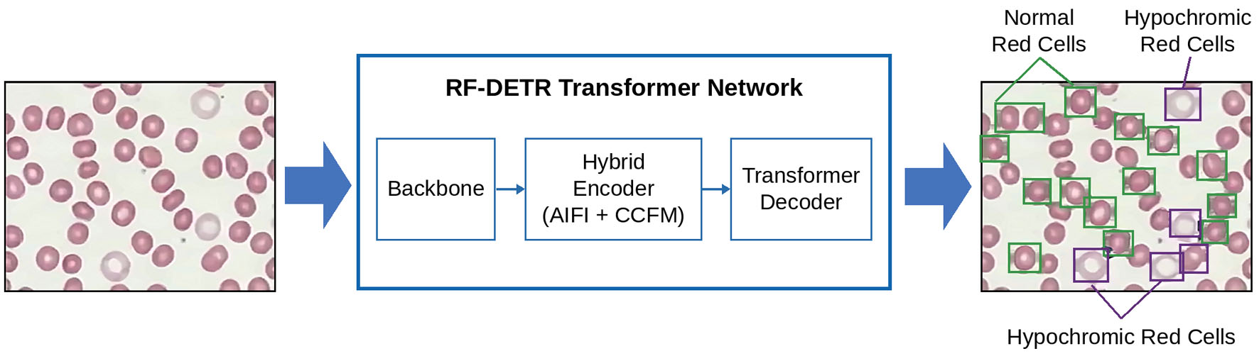
↓ Figure 1. RF-DETR neural network image analysis pipeline. A tiled peripheral blood smear image is passed through the RF-DETR transformer network, comprising a convolutional backbone for local feature extraction, a hybrid encoder (AIFI + CCFM) for multi-scale feature fusion, and a transformer decoder that outputs instance segmentation masks classifying each red blood cell as hypochromic or normochromic.
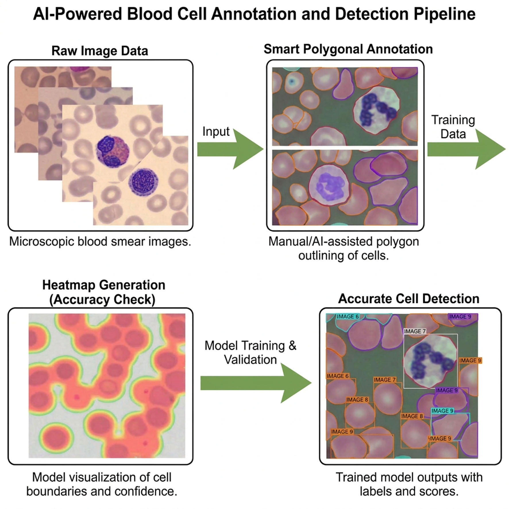
↓ Figure 2. The annotation process using smart polygonal instance segmentation. Overview of the AI-powered blood cell annotation and detection pipeline. Raw microscopic blood smear images undergo smart polygonal annotation (manual/AI-assisted polygon outlining of cells), model training with heatmap-based accuracy checks, and produce final trained-model outputs with confidence-scored cell detections.
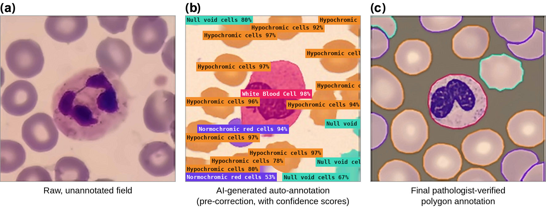
↓ Figure 3. Comparison of annotation stages on a representative peripheral blood smear field. (a) Raw, unannotated microscopic field of view. (b) AI-generated auto-annotation prior to pathologist correction, showing per-cell class predictions with confidence scores (hypochromic, normochromic, white blood cell, null/void). (c) Final pathologist-verified polygon annotation.
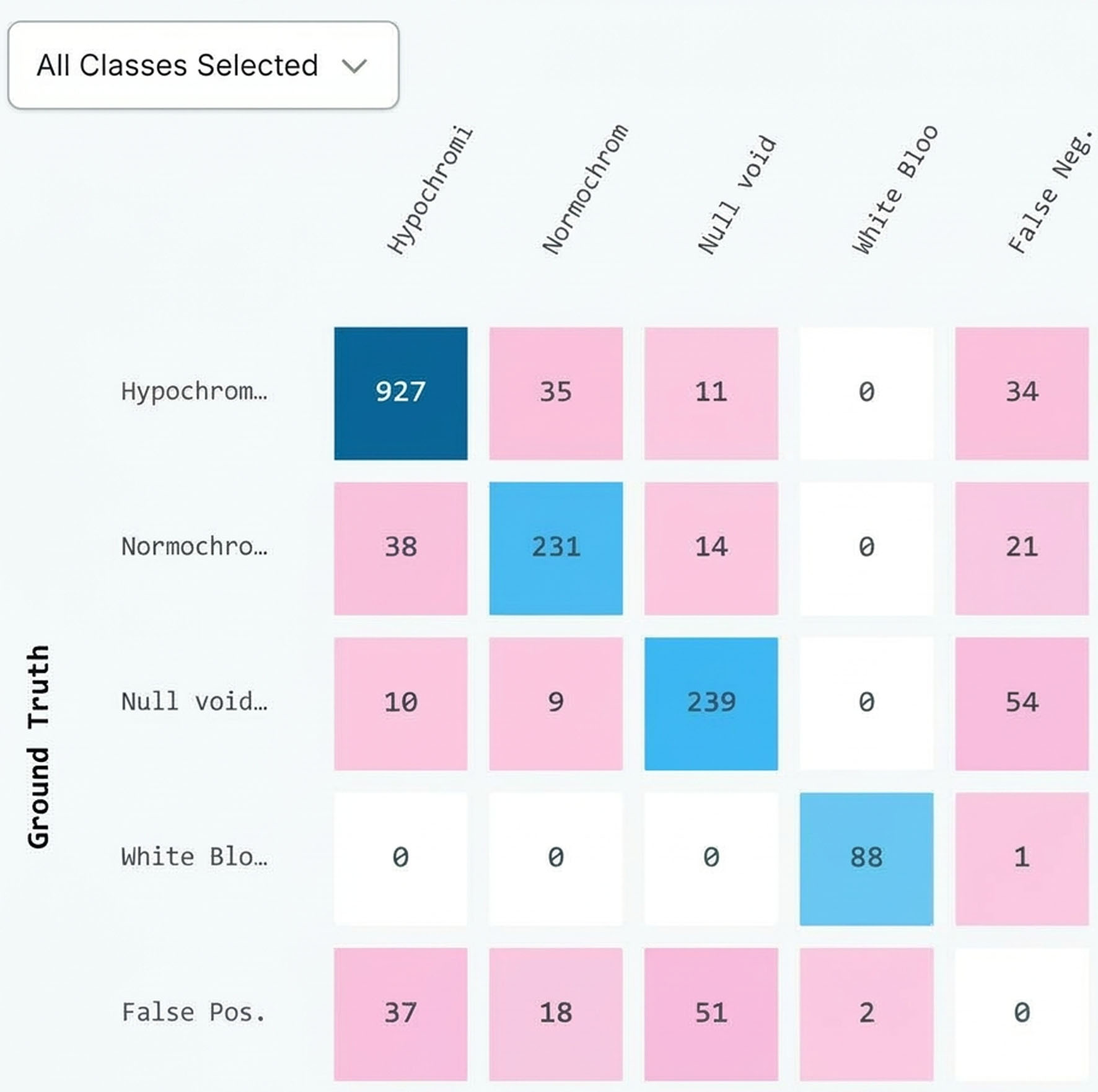
↓ Figure 4. Confusion matrix. Rows represent pathologist-verified ground-truth class; columns represent the model’s predicted class. Diagonal cells (dark blue/teal) indicate correct classifications; off-diagonal cells (pink) indicate misclassifications between classes. The “False Neg.” column records ground-truth cells the model failed to detect at all; the “False Pos.” row records model detections that did not correspond to any annotated cell. Cell values are raw counts from the held-out test set (n = 2,285 tiled images).
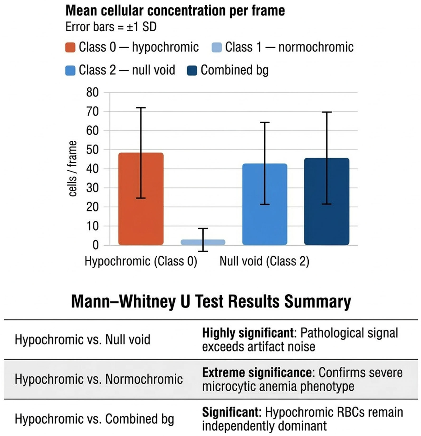
↓ Figure 5. Statistical analysis of the ANERBC 11 data subset used for validation (n = 600). Top: mean cell count per frame (± 1 SD, error bars) for hypochromic (Class 0), normochromic (Class 1), and null/void (Class 2) red blood cells, alongside the combined background (normochromic + null/void) count. Bottom: summary of pairwise Mann–Whitney U test results, indicating that the hypochromic count significantly exceeds each comparator population.
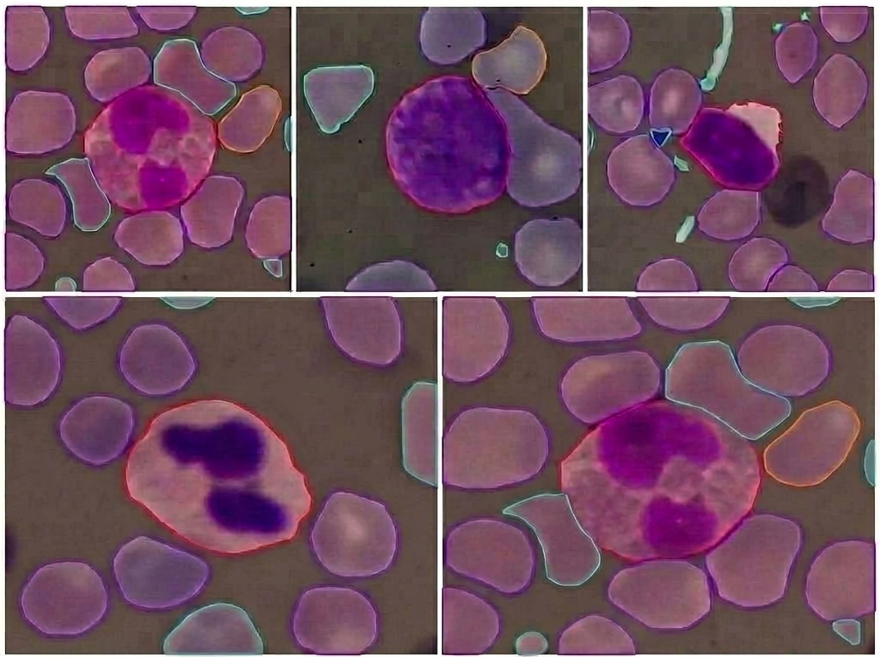
↓ Figure 6. Challenging edge cases encountered during annotation that required expert pathologist adjudication. Common ambiguous scenarios include: Borderline hypochromia—RBCs with subtle or incomplete central pallor (∼30–33% diameter) falling between normochromic and hypochromic classification thresholds; Overlapping/clustered cells—rouleaux formations or densely packed fields where individual cell boundaries are obscured, requiring careful segmentation to avoid merged instances; Out-of-focus regions—cells at the periphery of the focal plane exhibiting blurred boundaries that complicate precise mask delineation; Staining artifacts—precipitate, debris, or uneven Wright-Giemsa staining; Atypical cell morphologies—in particular unusual shaped cells due to adjacent crush effect. The model’s active learning algorithm prioritized these uncertain cases for pathologist-in-the-loop correction, enabling iterative refinement of decision boundaries.
Table
↓ Table 1. Summary of Model Performance and Validation Results
| Metric category | Parameter | Value/result | 95% CI |
|---|
| 95% confidence intervals were calculated using the Wilson score method for proportions with a defined numerator and denominator; a dash (—) indicates a metric for which a binomial confidence interval is not directly applicable (e.g., mAP, F1-score, mean ± SD values, and P-values). Reliability: The model demonstrated high discriminative power between leukocytes and erythrocytes, with zero misclassifications between the two groups. Statistical robustness: Mann–Whitney U testing confirmed that hypochromic RBCs are the dominant and statistically separable phenotype (P < 0.001) compared to normochromic cells and artifacts. Edge case analysis: Error analysis revealed that false negatives (n = 6) were primarily confined to the 20% hypochromic ratio boundary, suggesting that inaccuracies are limited to marginal “borderline” cases rather than systemic detection failures. |
| Global detection (mAP@50) | Overall accuracy | 90.0% | — |
| Primary performance metrics | Precision | 86.0% | 85.2–88.4% |
| Recall (sensitivity) | 85.9% | 85.1–88.3% |
| F1-score | 85.9% | — |
| Class-specific accuracy (TP) | Hypochromic red blood cells (RBCs) | 92.0% (927/1,007) | 90.2–93.6% |
| White blood cells (WBC) | 98.8% (88/89) | 93.9–99.8% |
| Optimization parameters | Optimal confidence threshold | 47% | — |
| Sensitivity/PPV at Threshold | 86%/86% | — |
| External validation (ANERBC II) | Sensitivity (IDA cohort) | 99% (594/600) | 97.8–99.5% |
| Hypochromic RBCs per frame | 48.31 ± 23.79 | — |
| Normochromic RBCs per frame | 2.88 ± 5.85 | — |
| Statistical significance | Hypochromic vs. normochromic | P = 9.61 × 10−182 | — |
| Hypochromic vs. background | P = 0.005 | — |