| AI in Clinical Medicine, ISSN 2819-7437 online, Open Access |
| Article copyright, the authors; Journal compilation copyright, AI Clin Med and Elmer Press Inc |
| Journal website https://aicm.elmerpub.com |
Original Article
Volume 2, 2026, e38

Fidelity, Robustness, and Plausibility of Post-Hoc Explanations for Diabetic Retinopathy Grading: An Empirical Application of the Clinical-Explainable Artificial Intelligence Evaluation Framework
Ali Alhazmia, b, c 
aDepartment of Computer Science, College of Engineering and Computer Science, Jazan University, Jazan, Saudi Arabia
bEngineering and Technology Research Center, Jazan University, PO Box 114, Jazan 82817, Saudi Arabia
cCorresponding Author: Ali Alhazmi, Department of Computer Science, College of Engineering and Computer Science, Jazan University, PO Box 114, Jazan 82817, Saudi Arabia
Manuscript submitted August 29, 2026, accepted October 20, 2026, published online November 13, 2026
Short title: Clinical-XAI Framework: Empirical Validation
doi: https://doi.org/10.14740/aicm38
| Abstract | ▴Top |
Background: A recent critical review proposed a six-dimension Clinical-explainable artificial intelligence (XAI) Evaluation Framework (fidelity, robustness, plausibility, actionability, equity, and regulatory readiness) for judging whether XAI methods are clinically adequate, but the framework itself was not empirically tested. This study examined whether three of these dimensions can be measured from real post-hoc explanations of a diabetic retinopathy (DR) grading model, how Gradient-weighted Class Activation Mapping (Grad-CAM), Local Interpretable Model-agnostic Explanations (LIME), and SHapley Additive exPlanations (SHAP) compare under a matched protocol, and whether the comparison holds across training runs and architectures.
Methods: Compact convolutional neural networks (CNNs) were trained from scratch with five random seeds, and a ResNet-18 comparator with three seeds, on RetinaMNIST (1,600 fundus images at 64 × 64 pixels, five severity grades). Grad-CAM, LIME, and SHAP were applied to the same 40 test images (eight per grade) with the same three Gaussian noise realizations (standard deviation (SD): 0.05 on a 0–1 intensity scale) and fixed explainer seeds. Fidelity was measured with deletion/insertion curves compared against random and center-prior pixel rankings, together with model-randomization sanity checks for all three methods. Robustness was the Spearman correlation between clean and noisy explanation maps, at native resolution and after pooling every map to 4 × 4. A background-attention check compared each map’s share of attribution inside the fundus disk with that image’s own disk-area share. Results are given with 95% bootstrap confidence intervals (CIs).
Results: The primary classifier reached 52.0% accuracy and a quadratic weighted kappa (QWK) of 0.624 (five-seed mean 50.0±3.0% and 0.582 ± 0.046). Fidelity exceeded the random-ranking baseline for Grad-CAM (paired difference 0.045, 95% CI 0.033 to 0.058) and SHAP (0.038, 0.028 to 0.050) but not for LIME (0.003, −0.004 to 0.010). At native0 resolution, Grad-CAM explanations were the most stable under noise (Spearman ρ 0.786), followed by SHAP (0.254) and LIME (0.097); after pooling to 4 × 4, SHAP (0.739) was comparable to Grad-CAM (0.767), whereas LIME remained unstable (0.171). The noise changed the predicted class in 53% of perturbed images. Grad-CAM passed the model-randomization check (ρ −0.120); LIME (0.335) and SHAP (0.386) retained partial similarity to explanations of a randomized model. All three methods placed more attribution inside the fundus disk than expected from its area. These findings were consistent across two CNN training seeds; see Section “Consistency across seeds and architectures” for the ResNet-18 comparator.
Conclusion: Fidelity, robustness, and a background-attention check can be measured directly from a trained model, but their interpretation depends on controls: a random-ranking baseline showed that LIME’s fidelity was indistinguishable from chance, and a resolution-matched analysis showed that most of Grad-CAM’s robustness advantage over SHAP reflects its coarse spatial resolution. Because small input noise often changed the model’s prediction, explanation stability cannot be interpreted separately from classifier reliability. The background-attention check is not a measure of clinical plausibility, which requires lesion-level annotation or ophthalmologist review. Actionability, equity, and regulatory readiness could not be assessed with this benchmark and require deployment data, subgroup metadata, or documentation review.
Keywords: Explainable artificial intelligence; Diabetic retinopathy; Deep learning; Medical imaging; Evaluation framework; Grad-CAM; SHAP; LIME
| Introduction | ▴Top |
Explainable artificial intelligence (XAI) is routinely proposed as a precondition for clinical trust in AI-assisted diagnosis, yet the methods used to generate explanations, saliency maps, feature-attribution scores, and their variants [1], are far more often deployed than they are validated, despite long-standing arguments for building interpretability into a model’s architecture from the outset rather than explaining a black box after the fact [2]. A recent critical review synthesized evidence across radiology, digital pathology, dermatology, and ophthalmology and proposed an integrated Clinical-XAI Evaluation Framework spanning six dimensions: fidelity, robustness, plausibility, actionability, equity, and regulatory readiness [3]. That review argued the field lacks a shared protocol for judging when an explanation is clinically adequate, and offered the six-dimension framework as one candidate protocol. What the review could not do, being a synthesis of existing literature rather than a new experiment, is show what happens when the framework is actually applied to a real model, real explanations, and real data.
This study addresses that gap. It trains classifiers for diabetic retinopathy (DR) severity grading, the single strongest empirical case in the originating review’s own account of inherently interpretable architectures [3], generates Gradient-weighted Class Activation Mapping (Grad-CAM), Local Interpretable Model-agnostic Explanations (LIME), and SHapley Additive exPlanations (SHAP) explanations for their predictions, and scores those explanations against three of the framework’s six dimensions using protocols that can be run on a public benchmark without a clinical deployment or a panel of ophthalmologists. Four research questions (RQs) were specified. RQ1 (fidelity): do the regions that each method ranks as important affect the model’s output more than regions chosen by random or center-weighted rankings, and do the explanations change when the model’s learned weights are randomized? RQ2 (robustness): how stable is each method’s explanation under a defined small input perturbation, and how much of any difference between methods is explained by the spatial resolution at which explanations are produced? RQ3 (background attention): does each method concentrate attribution inside the fundus field of view more than expected from the area of that field alone? RQ4 (consistency): do the answers to RQ1–RQ3 hold across independently trained models and a second network architecture? RQ3 is deliberately narrower than clinical plausibility, which would require lesion-level ground truth or expert review. The remaining three dimensions, actionability, equity, and regulatory readiness, are stated as outside this study’s scope rather than approximated with a weak proxy, since a false positive validation of a dimension the study design cannot actually test would defeat the framework’s purpose.
DR is a natural case for this test. It is a leading cause of preventable blindness and disproportionately affects populations with high diabetes prevalence; the Gulf Cooperation Council (GCC) region, including Saudi Arabia, has among the highest reported diabetes prevalence rates worldwide, estimated at 8–22% of adults across GCC countries by International Diabetes Federation data [4]. AI-assisted retinal screening has moved from research demonstration to regulatory deployment, including the first autonomous AI diagnostic system authorized by the US Food and Drug Administration (FDA) in any medical specialty [5], built on earlier work establishing that deep convolutional networks could match ophthalmologist-level accuracy for detecting referable DR in color fundus photographs [6]. This trajectory makes empirical evidence about whether such systems’ explanations can be trusted, not just whether their predictions are accurate, directly relevant to regional health-system interest in AI-assisted screening. The public dataset used here is not Saudi-sourced, a limitation stated explicitly in Section “Limitations”; the epidemiological motivation is regional even where the training data are not.
The remainder of this paper is organized as follows. The second section describes the dataset, models, explanation methods, and evaluation protocols. The third section reports classifier performance; fidelity, sanity-check, robustness, and background-attention results for the primary model; and the consistency of these results across training seeds and architectures. The fourth section interprets the findings, the fifth section outlines the limitations, and the sixth section states the conclusions.
| Materials and Methods | ▴Top |
Dataset
This study used RetinaMNIST, a component of the MedMNIST v2 benchmark collection [7], at its 64 × 64-pixel resolution. RetinaMNIST is derived from the DeepDRiD (Diabetic Retinopathy—Grading and Image Quality Estimation Challenge) dataset [8] and comprises 1,600 retinal fundus images labeled on a five-level ordinal severity scale (0 = no retinopathy through 4 = proliferative retinopathy), split by the benchmark’s own protocol into 1,080 training, 120 validation, and 400 test images. The dataset is released under a CC BY 4.0 license. Class distribution is imbalanced, consistent with the underlying clinical population, across all three splits (Table 1). File integrity was verified against the published Message-Digest Algorithm 5 (MD5) checksum before use. Pixel intensities were scaled to the 0–1 range. Channel-wise standardization (using training-set means and standard deviations (SDs)) was implemented as the first layer of each network, so that every explanation method operated on, and every perturbation was applied to, images in the same 0–1 pixel space.
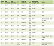 Click to view | Table 1. RetinaMNIST Dataset Composition by Split and Diabetic Retinopathy Severity Grade |
Classifier architecture and training
The primary classifier was a compact convolutional neural network (CNN) trained from scratch in PyTorch [9]: four convolutional blocks (32, 64, 128, and 256 channels; each a 3 × 3 convolution followed by batch normalization, rectified linear unit (ReLU) activation, and 2 × 2 max pooling), then global average pooling, dropout (P = 0.4), and a linear layer with five outputs (390,661 parameters). No pretrained weights were used. Training used class-weighted cross-entropy (weights inversely proportional to class frequency), the Adam optimizer (learning rate (LR) 10−3, weight decay 10−4, batch size 64), a scheduler that halved the LR after 8 epochs without improvement in validation loss, and light augmentation (horizontal flip with probability 0.5; rotation by 90°, 180°, or 270° with probability 0.3). Training ran for up to 150 epochs with early stopping after 25 epochs without improvement in validation quadratic weighted kappa (QWK) [10], the standard agreement measure for ordinal DR grading; the checkpoint with the highest validation QWK was retained. To quantify run-to-run variability, the same configuration was trained with five random seeds (42, 7, 123, 2024, and 31337). Seed 42 was designated in advance as the primary model for the detailed analyses, and all five models were evaluated with the identical explanation protocol. As an architectural comparator, a ResNet-18 (residual network) [11] was trained from scratch with the same procedure and three seeds (42, 7, and 123); its first convolution was changed to 3 × 3 with stride 2 and its initial max-pooling layer removed, so that its final feature map is also 4 × 4 for a 64 × 64 input (11.2 million parameters). The ResNet-18 seed-42 model was evaluated with the full explanation protocol. Table 2 summarizes the configuration.
Click to view | Table 2. Classifier Architectures and Training Configuration |
Explanation methods
Three widely used post-hoc explanation methods, the same three compared in the literature synthesized by the originating review [3], were applied to each model: Grad-CAM [12], LIME [13], and SHAP [14]. Grad-CAM was computed with the LayerGradCam implementation of the Captum library [15] on the output of the final convolutional block (a 4 × 4 map), with ReLU applied to the weighted activations and bilinear upsampling to 64 × 64; as a resolution ablation it was also computed on the penultimate block (an 8 × 8 map). LIME used the lime_image implementation with quickshift superpixel segmentation (kernel size 2, maximum distance 6, ratio 0.5; a median of 28 superpixels per image, interquartile range (IQR) 22–31), superpixels hidden by replacement with their mean color, 1,000 perturbation samples, and a fixed explainer seed; each pixel received the surrogate-model weight of its superpixel for the target class. SHAP used GradientExplainer (an expected-gradients approximation of SHapley values) with a fixed background of 32 training images, 200 samples per explanation, and a fixed seed; attributions were summed over the three color channels. Every explanation targeted the class predicted by the model for the clean image, and the same target was used for the noisy-input and randomized-model explanations, so that differences reflect the explanation rather than a change in explained class. Table 3 lists all settings and software versions.
Click to view | Table 3. Explanation-Method Settings, Evaluation Protocol, and Software Versions |
Explanations were generated for a fixed subset of 40 test images, eight per true severity grade, drawn at random with a fixed seed from each grade’s test images. The same 40 images were used for every method, model, and seed. The subset size was set by the computational cost of the matched protocol: each image requires, for each method, one clean explanation, three noisy-input explanations, two randomized-model explanations, a repeat explanation with a different explainer seed, and 65-point deletion and insertion curves. The whole protocol was run on central processing units (CPUs) only, at roughly 70 s per image per model. Equal stratification ensured that the rarest grade (Grade 4, 20 test images in total) contributed as many images as the most common grade, so that the results are not dominated by Grade 0.
Operationalizing three framework dimensions
Fidelity was assessed with a deletion/insertion protocol [16]. For each explanation, the 4,096 pixel positions were ranked by attribution value in descending order (signed values for LIME and SHAP, so that evidence for the target class ranks first; ties were broken by a fixed negligible random jitter). In 64 steps of 64 pixels, the deletion curve replaced the top-ranked pixels with the corresponding pixels of a Gaussian-blurred copy of the same image (blur SD 4 pixels), and the insertion curve started from the blurred image and progressively restored the original pixels. The model’s softmax probability for the target class was recorded at each of the 65 points, and the area under each curve (AUC) was computed with the trapezoidal rule over the fraction of pixels altered (0 to 1). The per-image combined fidelity score was (insertion AUC − deletion AUC + 1)/2; a value of 0.5 indicates that the ranking affects the output no more in one direction than the other, and higher values indicate that the highly ranked pixels drive the prediction. Because the absolute level of this score depends on the model and the perturbation, two reference rankings were scored on every image with the identical procedure: a random ranking (the mean of three random pixel orderings per image) and a center-prior ranking (pixels ordered by distance from the image center, a spatial baseline that requires no access to the model). The primary fidelity outcome was the per-image paired difference between each method’s score and the random-ranking score.
Robustness was assessed as explanation stability under a defined input perturbation: additive, independent Gaussian noise with SD σ = 0.05 on the 0–1 intensity scale (5% of the dynamic range, a peak signal-to-noise ratio of approximately 26 dB), applied per pixel and per color channel and clipped to [0, 1]. Three noise realizations per image were generated from fixed seeds and reused unchanged for every method, model, and seed. Explainer seeds were held fixed between the clean and noisy runs, so that only the input changed, and the explained class was held at the clean-image prediction. Stability was the Spearman rank correlation between the clean and noisy explanation maps, averaged over the three realizations to give one value per image. To separate stability from spatial resolution, the same correlation was also computed after average-pooling every map to 4 × 4, the native resolution of the final-layer Grad-CAM map. Because the perturbation can change the model’s prediction, whether the predicted class changed was recorded for every noisy image, and stability was reported separately for images whose prediction was unchanged in all three realizations and for the remaining images. For LIME and SHAP, which are stochastic, an explainer-seed floor was also computed: the Spearman correlation between two explanations of the same clean image generated with different explainer seeds (Grad-CAM is deterministic).
The automated plausibility proxy was a background-attention check. A fundus-disk mask was obtained for each image by thresholding channel-mean intensity at 15/255, followed by a one-iteration morphological opening (3 × 3 structuring element) and hole filling; this separates the circular field of view from the near-black padding around it (median disk-area share 0.700, IQR 0.664–0.732). For each explanation, the share of total absolute attribution falling inside the mask was compared with that image’s own disk-area share, and the paired per-image difference was the outcome; a positive value indicates that the explanation concentrates attribution in the field of view more than a spatially uniform map would. Maps with zero total attribution were excluded from this metric and counted, and Spearman correlations involving a constant map (undefined) were likewise excluded and counted in every analysis. This check tests only whether an explanation avoids attending to background or padding. It does not test whether an explanation highlights clinically relevant pathology such as microaneurysms, hemorrhages, or exudates, which requires lesion-level annotations or a blinded reader study with ophthalmologists, and it is therefore not reported as a measure of clinical plausibility.
Actionability, equity, and regulatory readiness, the framework’s remaining three dimensions, were not scored in this study. Actionability requires measuring a change in clinician behavior or patient outcome under real or simulated deployment; equity requires demographic subgroup metadata (for example, sex, age, ethnicity, or imaging device) that RetinaMNIST, a de-identified public benchmark, does not provide; and regulatory readiness requires assessment against a specific jurisdiction’s documentation and oversight requirements, which was outside the scope of this technical analysis. These omissions reflect the design and data of this particular study; they do not imply that retrospective studies in general cannot address these dimensions, for example, equity where subgroup metadata are available, or elements of regulatory readiness through documentation audits. Table 4 summarizes which of the six dimensions were tested, the protocol used, and why the remaining three were out of scope.
Click to view | Table 4. Coverage of the Six Clinical-XAI Evaluation Framework Dimensions in This Study |
Statistical analysis
Classifier performance was summarized with accuracy, macro-averaged F1-score, and QWK, alongside the confusion matrix and per-class precision, recall, and F1-score. For the explanation metrics the image was the unit of analysis. Means are reported with 95% percentile bootstrap confidence intervals (CIs) from 5,000 resamples of the 40 images, together with SDs where useful. Paired comparisons (each method against the random baseline, each method’s in-disk share against the image’s disk-area share, and pairwise method contrasts) used per-image differences with bootstrap CIs and two-sided Wilcoxon signed-rank tests; within each family of three method-level tests, P values were adjusted with the Holm procedure. Variability across training runs was summarized as the mean ± SD of the per-model means over the five CNN seeds. Analyses were implemented in Python 3.13 with the libraries and versions listed in Table 3.
Ethical considerations
The data analyzed here are RetinaMNIST, a de-identified benchmark released publicly for research and derived from the DeepDRiD challenge [8]. The author collected no data from human participants and had no access to identifiable patient information at any stage. Because the work is a secondary analysis of an anonymized public dataset, it did not constitute human-subjects research requiring new institutional review board approval. According to its providers, the original DeepDRiD data were collected in accordance with the ethical standards of the responsible institutions and the Declaration of Helsinki [8]; the author was not involved in that collection and cannot attest to its ethical review beyond what the source publication reports. No animals were involved.
| Results | ▴Top |
Classifier performance
The primary classifier (seed 42) reached 52.0% accuracy, a macro-averaged F1-score of 0.406, and a QWK of 0.624 on the 400-image test set; training stopped after 49 epochs, with the best validation QWK (0.704) at epoch 24. Across the five CNN seeds, accuracy was 50.0±3.0% (range 45.2–53.2%), macro F1 0.394 ± 0.036, and QWK 0.582 ± 0.046 (range 0.510–0.624); the three ResNet-18 models reached 50.4±0.4% accuracy and a QWK of 0.551 ± 0.025; therefore, the larger architecture did not improve performance on this small dataset. Table 5 gives per-class results for the primary model: performance was strongest for the majority class (Grade 0) and weaker for the minority grades, consistent with the class imbalance of the training set (486 Grade-0 images versus 66–206 for the other grades). Figure 1 shows the training curves: validation QWK rose until about epoch 24 and then plateaued, while validation loss increased as training loss continued to fall, indicating overfitting of a model trained from scratch on 1,080 images. Most errors in the confusion matrix (Fig. 2) occurred between adjacent grades, the expected pattern for an ordinal task and the one that QWK, unlike accuracy, penalizes in proportion to ordinal distance. The model was also not confident: on the 40 explained images the median softmax probability of the predicted class was 0.41 (IQR 0.35–0.59), and 19 of the 40 were classified correctly. These properties bound the interpretation of the explanation results that follow (Section “Explanation quality cannot be separated from classifier reliability”).
Click to view | Table 5. Per-Class Precision, Recall, and F1-Score for the Primary Classifier (CNN, Seed 42) on the 400-Image RetinaMNIST Test Set |
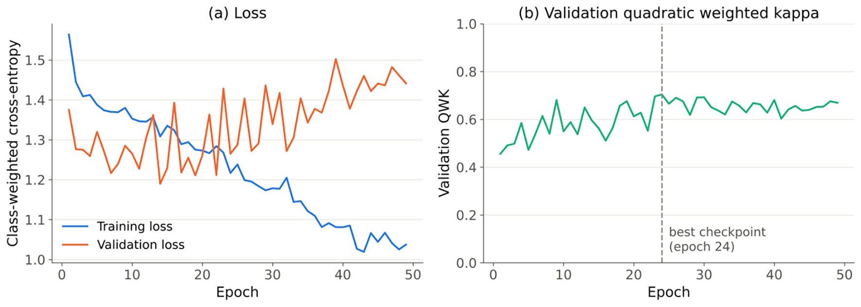 Click for large image | Figure 1. Training curves for the primary compact CNN (seed 42) trained from scratch on RetinaMNIST. (a) Class-weighted cross-entropy loss on the training and validation sets. (b) Validation quadratic weighted kappa; the dashed line marks the retained checkpoint. CNN: convolutional neural network. |
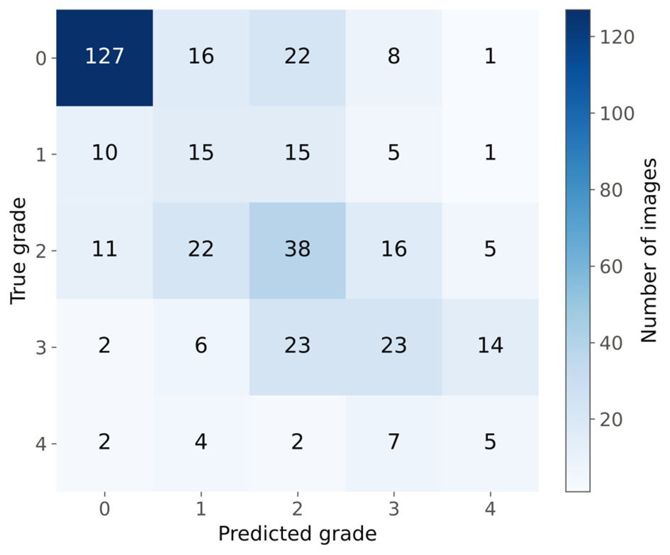 Click for large image | Figure 2. Confusion matrix of the primary CNN (seed 42) on the 400-image RetinaMNIST test set for five-level diabetic retinopathy grading (0 = no retinopathy to 4 = proliferative retinopathy). CNN: convolutional neural network. |
Fidelity and sanity checks
Deletion and insertion curves for the primary model are shown in Figure 3, and per-image results in Figure 4a and Table 6. Grad-CAM and SHAP produced steeper deletion curves and higher insertion curves than the random ranking. Their combined fidelity scores were 0.545 (95% CI 0.534, 0.558) and 0.538 (95% CI 0.528, 0.550), against 0.500 for the random ranking and 0.513 for the center-prior ranking. The paired advantage over the random ranking was 0.045 (95% CI 0.033, 0.058) for Grad-CAM (P < 0.001, Holm-adjusted; positive in 39 of 40 images) and 0.038 (95% CI 0.028, 0.050) for SHAP (P < 0.001; positive in 38 of 40). Both methods also exceeded the center-prior ranking (Grad-CAM 0.032 (95% CI 0.020, 0.045); SHAP 0.025 (95% CI 0.008, 0.043)). LIME’s fidelity score (0.504 (95% CI 0.497, 0.510)) was indistinguishable from the random ranking (paired difference 0.003 (95% CI −0.004, 0.010), P = 0.36) and from the center-prior ranking (−0.009 (95% CI −0.027, 0.007)). The penultimate-layer Grad-CAM map (8 × 8) scored 0.556 (95% CI 0.543, 0.572). All differences were small in absolute terms: across all curves the mean predicted-class probability varied only between 0.41 and 0.55 (Fig. 3), which reflects the model’s low confidence.
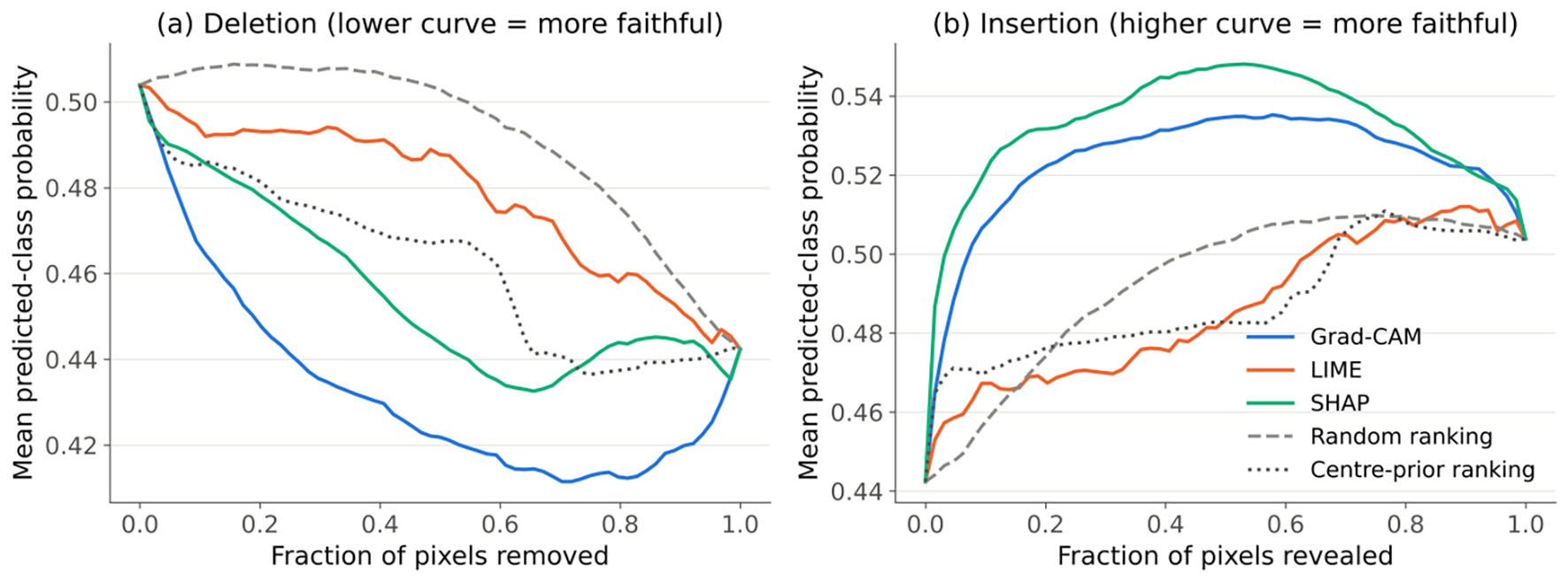 Click for large image | Figure 3. Figure 3. Deletion (a) and insertion (b) curves for the primary CNN (seed 42), averaged over the 40 explained test images. The curves show the mean softmax probability of the target (predicted) class as pixels are progressively replaced by a blurred copy of the image (deletion) or restored from it (insertion), in the order given by Grad-CAM, LIME, or SHAP, or by the random and center-prior reference rankings. CNN: convolutional neural network; Grad-CAM: Gradient-weighted Class Activation Mapping; LIME: Local Interpretable Model-agnostic Explanations; SHAP: SHapley Additive exPlanations. |
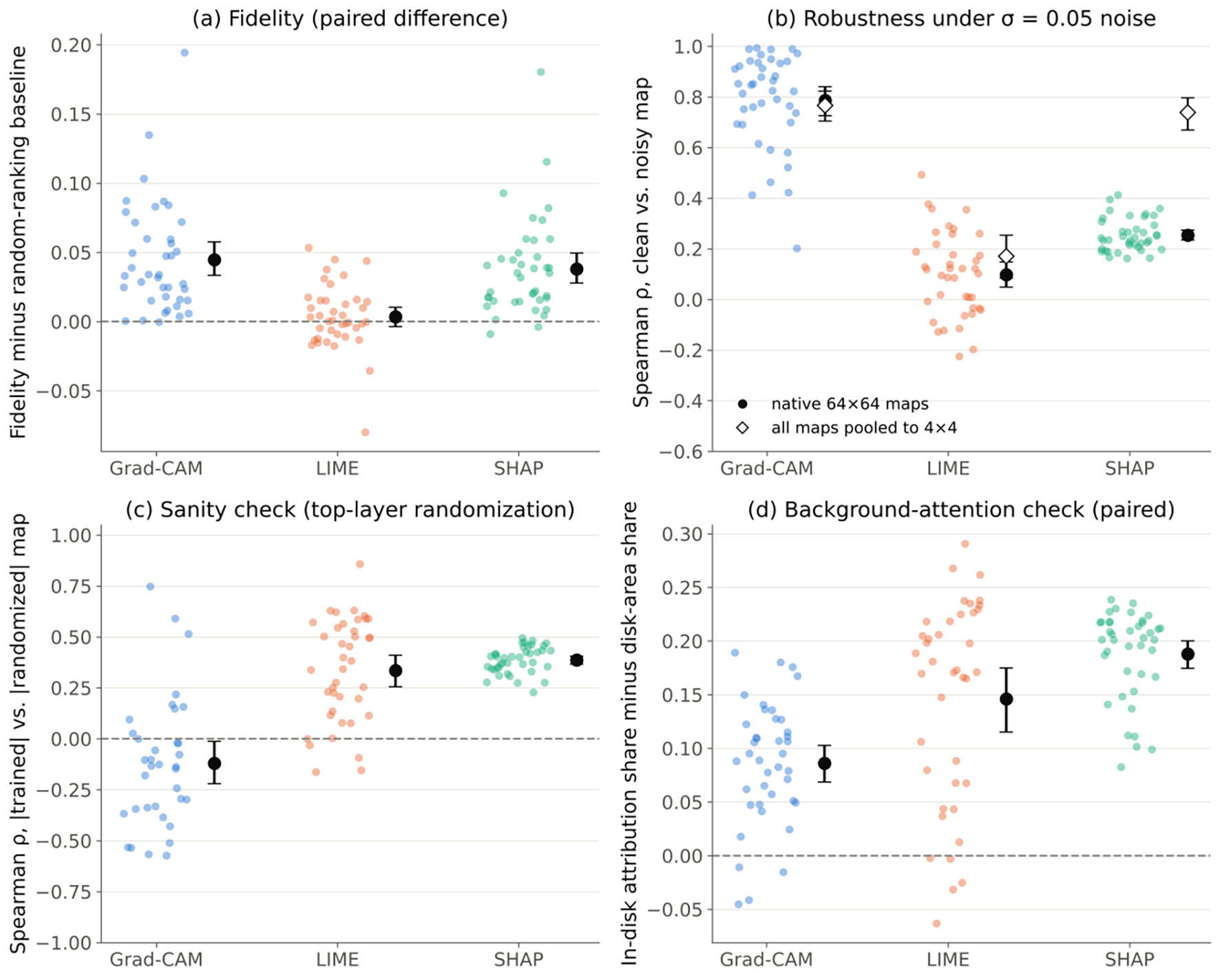 Click for large image | Figure 4. Per-image explanation metrics for the primary CNN (seed 42; n = 40 images). Dots are individual images; black markers and bars are means with 95% bootstrap confidence intervals. (a) Combined deletion/insertion fidelity score minus the random-ranking score of the same image. (b) Spearman correlation between clean and noisy explanation maps (σ = 0.05), averaged over three noise realizations; open diamonds give the same statistic after pooling all maps to 4 × 4. (c) Spearman correlation between absolute-value maps from the trained model and from a model with re-initialized top layers; the five images for which the randomized Grad-CAM map was all zero are not shown. (d) Share of absolute attribution inside the fundus disk minus the disk’s share of the image area. Dashed lines mark zero difference. CNN: convolutional neural network; Grad-CAM: Gradient-weighted Class Activation Mapping; LIME: Local Interpretable Model-agnostic Explanations; SHAP: SHapley Additive exPlanations. |
Click to view | Table 6. Fidelity, Sanity-Check, Robustness, and Background-Attention Results for the Primary Model, by Explanation Method |
In the model-randomization sanity check [17], explanations from the trained model were compared with explanations of the same image and target class from models whose top layers (final convolutional block and classification layer), or all layers, had been re-initialized. Grad-CAM maps showed no positive correspondence with their top-randomized counterparts (mean Spearman ρ −0.120 (95% CI −0.221, −0.013); n = 35, with five images excluded because the randomized model produced an all-zero map), which is the expected behavior of an explanation that depends on learned weights. With full randomization, 18 of the 40 randomized Grad-CAM maps were all zero after the ReLU; the remaining 22 gave ρ = 0.269 (95% CI 0.140, 0.386). LIME (top: 0.335 (95% CI 0.255, 0.411); full: 0.357 (95% CI 0.271, 0.437)) and SHAP (top: 0.386 (95% CI 0.366, 0.406); full: 0.311 (95% CI 0.291, 0.331)) retained a moderate positive correlation with the randomized-model explanations. Because the corresponding explainer-seed floors were high (LIME 0.991; SHAP 0.935), this residual similarity cannot be attributed to explainer stochasticity. It indicates that part of the spatial structure of the LIME and SHAP maps is driven by the input image rather than by what the model learned. These two methods therefore passed the check only partially (Fig. 4c).
Robustness
Robustness results are shown in Figure 4b and Table 6. At native resolution, Grad-CAM explanations were the most stable under noise (mean Spearman ρ 0.786 (95% CI 0.726, 0.840)), SHAP was markedly less stable (0.254 (95% CI 0.235, 0.274)), and LIME was least stable (0.097 (95% CI 0.048, 0.149)); all pairwise differences were significant (Grad-CAM minus SHAP 0.532 (95% CI 0.472, 0.586), P < 0.001). When every map was pooled to 4 × 4, SHAP’s stability rose to 0.739 (95% CI 0.670, 0.797) and no longer differed from Grad-CAM’s (0.767 (95% CI 0.704, 0.823); difference 0.028 (95% CI −0.047, 0.110), P = 0.64). LIME remained unstable even after pooling (0.171 (95% CI 0.084, 0.254)). The 8 × 8 penultimate-layer Grad-CAM map was less stable than the 4 × 4 final-layer map (0.687 (95% CI 0.608, 0.760)). The perturbation was not negligible for the classifier: it changed the predicted class in 53% of the 120 noisy images, and only 18 of the 40 images kept their predicted class in all three realizations. Stability was higher in these 18 images than in the other 22 for Grad-CAM (0.871 vs. 0.716) and SHAP (0.296 vs. 0.219), but not for LIME (0.092 vs. 0.102). Explainer-seed floors were 0.991 for LIME and 0.935 for SHAP; therefore, the instability under noise was not caused by the explainers’ own sampling.
Background-attention check
All three methods placed more absolute attribution inside the fundus disk than expected from the disk’s area (Fig. 4d, Table 6). The mean paired difference between the in-disk share and the image’s own disk-area share was 0.188 (95% CI 0.174, 0.200) for SHAP (positive in 40 of 40 images), 0.146 (95% CI 0.115, 0.175) for LIME (positive in 35 of 40), and 0.086 (95% CI 0.069, 0.103) for Grad-CAM (positive in 36 of 40); all Holm-adjusted P < 0.001. No map had zero total attribution. Figure 5 shows explanations for three test images. Two features of these examples illustrate the limits of the check. First, Grad-CAM’s map is coarse because it is upsampled from a 4 × 4 feature map. Second, SHAP repeatedly assigned strong attribution to a bright arc at the lower edge of the field of view (arrows in Fig. 5), an acquisition artifact that lies at the disk boundary and is therefore largely counted as in-disk attention.
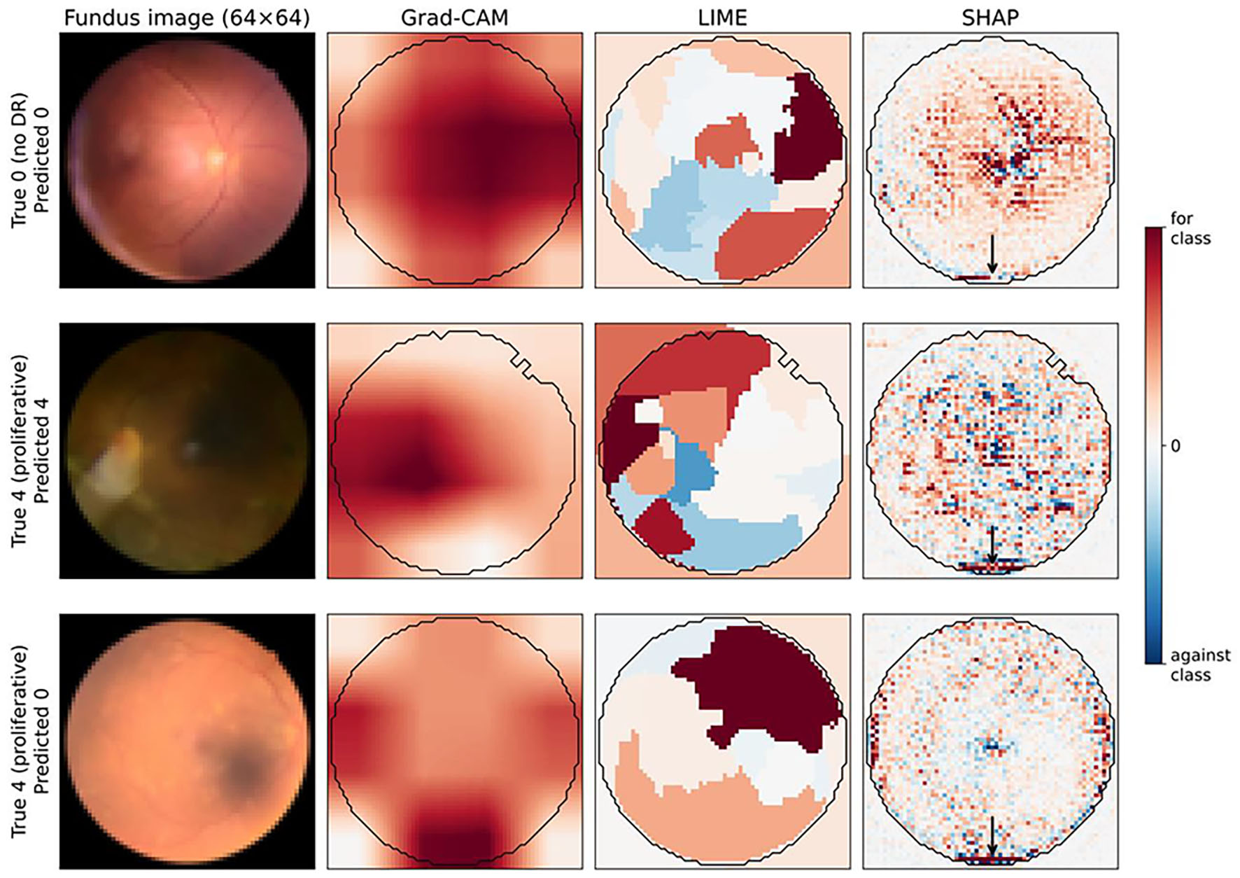 Click for large image | Figure 5. Grad-CAM, LIME, and SHAP explanations from the primary CNN (seed 42) for three RetinaMNIST test images: a correctly classified Grade 0 image, a correctly classified Grade 4 image, and a Grade 4 image misclassified as Grade 0. Red indicates evidence for the predicted class and blue evidence against it; each map is scaled to its own 99th percentile of absolute attribution. The black contour is the automatically derived fundus-disk mask used in the background-attention check. Arrows mark SHAP attribution concentrated on the bright arc at the lower edge of the field of view, an image-acquisition artifact. Images are 64 × 64 pixels and contain no patient-identifying marks. CNN: convolutional neural network; Grad-CAM: Gradient-weighted Class Activation Mapping; LIME: Local Interpretable Model-agnostic Explanations; SHAP: SHapley Additive exPlanations. |
Consistency across seeds and architectures
The CNN seeds were all evaluated with the identical protocol (Table 7). The fidelity advantage of Grad-CAM and SHAP over the random ranking, with 95% CIs excluding zero, was found for two of two seeds, and LIME’s fidelity was indistinguishable from the random ranking (CI including zero) for two of two seeds. The native-resolution robustness ordering Grad-CAM > SHAP > LIME held for two of two seeds. After pooling to 4 × 4, the Grad-CAM–SHAP difference had a CI including zero for two of two seeds, and LIME was the least stable method for two of two seeds. Grad-CAM had the lowest top-layer sanity-check correlation for two of two seeds, and all three methods exceeded the disk-area baseline (all CIs above zero) for two of two seeds. The noise perturbation changed the predicted class in 46–53% of noisy images across seeds.
Click to view | Table 7. Consistency of Explanation Metrics Across Training Seeds and Architectures |
| Discussion | ▴Top |
Fidelity was measurable but modest, and is not comparable across metric definitions
Against a random-ranking control, Grad-CAM and SHAP showed small but consistent fidelity, whereas LIME did not. Without this control, the three raw fidelity scores (0.50–0.55) would have suggested a narrow spread between similar methods; with it, LIME’s score is seen to be indistinguishable from chance. The small absolute margins have a concrete cause: the model’s predicted-class probabilities were low and changed little as pixels were removed or restored (Fig. 3); therefore, any ordering of pixels can shift the output by only a small amount. Fidelity estimates for a weak model are therefore compressed toward the baseline, which is one reason why fidelity should be reported relative to explicit reference rankings rather than as an absolute number.
The originating review cited a meta-analysis that ranked LIME well above Grad-CAM and SHAP on fidelity [18]. The present results do not reproduce that ordering, but the two sets of numbers should not be compared numerically. In that meta-analysis, fidelity was defined as the correlation between attribution scores and the change in prediction under occlusion and was pooled across heterogeneous studies, architectures, and modalities, whereas the present score is a deletion/insertion area difference computed for single models on one dataset. Because the two definitions are not equivalent and no calibration between them is available, a numerical comparison of the two sets of scores would not be meaningful. The qualitative point that remains is the one the framework makes: fidelity is a property of a method applied to a particular model and task; therefore, it must be re-established for each application rather than inherited from the literature [3, 19].
Grad-CAM’s robustness advantage largely reflects its spatial resolution
At native resolution Grad-CAM appeared far more robust than SHAP, but the resolution-matched analysis showed that this advantage largely disappears when both are compared on the same 4 × 4 grid. The final-layer Grad-CAM map is computed from a 4 × 4 feature map and smoothly upsampled; therefore, it has little capacity to change at the pixel level, whereas SHAP assigns a separate value to every pixel and inherits pixel-level noise directly. Two further observations support this interpretation. First, the 8 × 8 penultimate-layer Grad-CAM map was less stable than the 4 × 4 map, which is the expected direction if coarseness itself confers stability. Second, SHAP’s stability rose from 0.254 to 0.739 after pooling, while Grad-CAM’s barely changed. A high native-resolution robustness score earned through coarseness says little about whether an explanation is faithful or useful, and Grad-CAM did not lead correspondingly on fidelity, where it and SHAP were similar. This is the kind of interaction between dimensions that the framework’s multi-dimensional design is meant to expose, and it argues for reporting robustness at a stated, matched resolution and for reading each dimension alongside the others rather than collapsing them into one composite score [3].
LIME’s instability persists after resolution matching
LIME was unstable at both native and pooled resolution, and its explainer-seed floor (0.991) shows that its own sampling was not the cause. The most plausible mechanism is the superpixel segmentation: quickshift is recomputed on the noisy image, and on a 64 × 64 image with about 28 superpixels, small intensity changes move segment boundaries enough to change which regions the surrogate model weighs. This interpretation is consistent with LIME’s stability being similar whether or not the prediction changed. It is a statement about LIME with input-dependent segmentation on low-resolution images, not about LIME in general; fixing the segmentation across perturbations, or using larger images in which segment boundaries are less sensitive to pixel noise, could change the result, and neither was tested here.
Explanation quality cannot be separated from classifier reliability
Noise with SD of 5% of the intensity range changed the predicted class for more than half of the perturbed images. This perturbation is therefore not negligible for this model. It also means that, for many images, the model’s internal evidence genuinely changed under noise; therefore, some loss of explanation stability is expected even for a perfectly faithful explainer. Stability was indeed higher in images whose prediction did not change, for Grad-CAM and SHAP. More generally, the classifier’s modest accuracy, low confidence, and sensitivity to noise limit what its explanations can show: a faithful explanation of an unreliable model is still an explanation of unreliable reasoning. For this reason, the explanation results here are best read as a demonstration that the three dimensions can be measured, and of how controls change their interpretation, rather than as evidence about explanations of a clinically deployable DR model. Repeating the protocol on higher-resolution images with a well-performing model is necessary before drawing conclusions about method choice in clinical screening.
Sanity checks and the limits of the background-attention check
Applying the sanity check to all three methods was informative: Grad-CAM passed, but LIME and SHAP retained a moderate correlation with explanations of randomized models. This is consistent with earlier findings that gradient- and perturbation-based attributions can partly reflect image structure independent of the model’s learned parameters [17]. The background-attention check, by contrast, was passed by all three methods, and SHAP passed it most strongly, yet Figure 5 shows SHAP attending to an acquisition artifact at the edge of the field of view. A method can therefore pass this check while attending to clinically irrelevant structure, and the check should be read only as evidence against gross attention to padding. Genuine plausibility assessment requires lesion-level ground truth, such as the pixel-level annotations of microaneurysms, hemorrhages, and exudates in the Indian Diabetic Retinopathy Image Dataset (IDRiD) [20], or a blinded reader study with ophthalmologists. A broader perspective is also relevant. Retinal images carry information beyond DR lesions, including signals associated with systemic disease and cardiovascular risk factors [21, 22], and foundation models trained on large collections of retinal images, increasingly combined with other modalities such as optical coherence tomography (OCT), are changing what a retinal classifier relies on [23]. For such models and multimodal diagnostic pipelines, plausibility will have to be judged against a wider and less settled set of retinal imaging biomarkers than lesion maps alone, which makes explicit, quantitative evaluation of explanations more important rather than less.
What this study establishes, and what it does not
This study shows that three of the framework’s six dimensions (fidelity, robustness, and a background-attention check as a partial stand-in for plausibility) can be measured directly from trained models and their explanations, without a clinical deployment or an expert panel. It also shows that the controls matter as much as the metrics: random and spatial reference rankings, sanity checks applied to every method, resolution-matched comparison, matched noise realizations, and replication across seeds each changed or qualified a conclusion that the uncontrolled analysis would have suggested. It does not establish that Grad-CAM, LIME, or SHAP is the better choice for DR screening, because the classifiers were weak, the images low-resolution, and the dataset small. It deliberately tested post-hoc explanation of black-box classifiers rather than inherently interpretable architectures; other work on DR has shown that models in which explanation and prediction are unified by construction can match black-box accuracy while producing structurally faithful evidence maps [24, 25]. The post-hoc design was chosen not to displace that approach but because post-hoc explanation of an existing black-box model remains the more common, and more contested, case in practice. Finally, the study says nothing about actionability, equity, or regulatory readiness, which it did not test (Section “Operationalizing three framework dimensions”), and the three tested dimensions should not be read as a proxy for the framework as a whole.
Limitations
Several limitations bound these conclusions. First, RetinaMNIST is small (1,600 images) and low-resolution (64 × 64), and the classifiers were trained from scratch because pretrained weights were not available in the computing environment; clinical-grade screening models use higher-resolution images, larger datasets, and usually transfer learning, and their explanations may behave differently. In particular, the resolution dependence of robustness, the instability of LIME’s segmentation, and the compression of fidelity scores observed here may all be weaker at clinical resolutions; therefore, the findings should not be extrapolated to clinical images. Second, the classifiers were not clinically reliable (accuracy about 50%, QWK about 0.58) and were sensitive to the noise used for the robustness test (Section “Explanation quality cannot be separated from classifier reliability”). Third, explanations were evaluated on 40 images per model. The bootstrap intervals show that this was sufficient to separate the methods on most metrics, but it limits subgroup analyses (for example, by severity grade). Fourth, although five CNN seeds and a second architecture were evaluated, the ResNet-18 was evaluated with only one seed, and other architectures, perturbation types (for example, blur or contrast changes), noise levels, and deletion baselines were not tested; fidelity scores in particular depend on the choice of replacement image. Fifth, the background-attention check is anatomical and coarse: it uses an intensity-threshold mask, counts boundary artifacts as in-disk attention, and does not assess whether explanations highlight DR lesions. Sixth, the dataset is not Saudi- or Gulf-sourced; the regional motivation in the introduction section explains why the question matters for GCC health systems, but the findings should not be assumed to transfer to Saudi patient populations, imaging equipment, or disease-prevalence profiles without local validation, a caveat the originating review raised for imported models generally [3].
Conclusions
Applying three of the six Clinical-XAI Evaluation Framework dimensions to trained DR classifiers under a matched protocol showed that the dimensions are measurable, and that their interpretation depends on controls. Grad-CAM and SHAP showed small but consistent fidelity relative to a random ranking, whereas LIME did not. Grad-CAM’s apparent robustness advantage over SHAP largely disappeared when explanations were compared at the same spatial resolution, and LIME was unstable at any resolution. Only Grad-CAM fully passed the model-randomization sanity check. All three methods passed a background-attention check, which, however, cannot detect attention to artifacts within the field of view and is not a test of clinical plausibility. Because small input noise often changed the classifier’s prediction, explanation quality must be read together with classifier reliability. These results support the framework’s premise that fidelity and robustness must be re-established for each application, and they suggest that evaluation reports should include reference rankings, sanity checks for every method, resolution-matched robustness, and replication across training runs. Future work should apply this protocol to higher-resolution clinical images and well-performing models, use lesion-level annotations and a blinded ophthalmologist reader study to test plausibility, and assess actionability, equity, and regulatory readiness using deployment studies, data with subgroup metadata, and documentation review.
Acknowledgments
None to declare.
Financial Disclosure
None. This study received no specific grant from any funding agency in the public, commercial, or not-for-profit sectors.
Conflict of Interest
The author declares no conflict of interest.
Informed Consent
Not applicable.
Author Contributions
As sole author, Ali Alhazmi conceived the study, trained the model, conducted the XAI analysis, drafted the manuscript, and approved the final version.
Data Availability
The trained model weights, analysis code, explanation maps, and per-image results supporting this study’s findings are available from the corresponding author upon reasonable request.
AI Use Declaration
During preparation of this manuscript, including its revision, the author used Claude (Anthropic) to assist with code implementation, literature search, and drafting of the manuscript text. The author directed the study design, ran and reviewed all analyses, and takes full responsibility for the content, computed results, citations, and conclusions presented. All cited sources were independently verified against their original publications. No AI tool is listed as an author, and no experimental results in this manuscript were generated or fabricated by an AI tool without the author’s direct execution and verification.
Abbreviations
AI: artificial intelligence; AUC: area under the curve; CI: confidence interval; CNN: convolutional neural network; CPU: central processing unit; DeepDRiD: Diabetic Retinopathy Grading and Image Quality Estimation Challenge Dataset; DR: diabetic retinopathy; F1: F1-score (harmonic mean of precision and recall); FDA: US Food and Drug Administration; GCC: Gulf Cooperation Council; Grad-CAM: Gradient-weighted Class Activation Mapping; IDRiD: Indian Diabetic Retinopathy Image Dataset; IQR: interquartile range; LIME: Local Interpretable Model-agnostic Explanations; LR: learning rate; MD5: Message-Digest Algorithm 5; OCT: optical coherence tomography; QWK: quadratic weighted kappa; ResNet: Residual Network; ReLU: rectified linear unit; RQ: research question; SD: standard deviation; SHAP: SHapley Additive exPlanations; XAI: explainable artificial intelligence
| References | ▴Top |
- Barredo Arrieta A, Diaz-Rodriguez N, Del Ser J, Bennetot A, Tabik S, Barbado A, et al. Explainable Artificial Intelligence (XAI): concepts, taxonomies, opportunities and challenges toward responsible AI. Inf Fusion. 2020;58:82-115.
- Rudin C. Stop explaining black box machine learning models for high stakes decisions and use interpretable models instead. Nat Mach Intell. 2019;1(5):206-215.
doi pubmed - Alhazmi A. Explainable AI in medical imaging and diagnosis: a critical review of methods, clinical translation barriers, and an integrated evaluation framework. AI Clin Med. 2026;2:e36.
doi - Aljulifi MZ. Prevalence and reasons of increased type 2 diabetes in Gulf Cooperation Council Countries. Saudi Med J. 2021;42(5):481-490.
doi pubmed - Abramoff MD, Lavin PT, Birch M, Shah N, Folk JC. Pivotal trial of an autonomous AI-based diagnostic system for detection of diabetic retinopathy in primary care offices. NPJ Digit Med. 2018;1:39.
doi pubmed - Gulshan V, Peng L, Coram M, Stumpe MC, Wu D, Narayanaswamy A, Venugopalan S, et al. Development and validation of a deep learning algorithm for detection of diabetic retinopathy in retinal fundus photographs. JAMA. 2016;316(22):2402-2410.
doi pubmed - Yang J, Shi R, Wei D, Liu Z, Zhao L, Ke B, Pfister H, et al. MedMNIST v2 - A large-scale lightweight benchmark for 2D and 3D biomedical image classification. Sci Data. 2023;10(1):41.
doi pubmed - Liu R, Wang X, Wu Q, Dai L, Fang X, Yan T, Son J, et al. DeepDRiD: diabetic retinopathy-grading and image quality estimation challenge. Patterns (N Y). 2022;3(6):100512.
doi pubmed - Paszke A, Gross S, Massa F, Lerer A, Bradbury J, Chanan G, Killeen T, et al. PyTorch: an imperative style, high-performance deep learning library. Adv Neural Inf Process Syst. 2019;32:8024-8035.
- Cohen J. Weighted kappa: nominal scale agreement with provision for scaled disagreement or partial credit. Psychol Bull. 1968;70(4):213-220.
doi pubmed - He K, Zhang X, Ren S, Sun J. Deep residual learning for image recognition. Proc IEEE Conf Comput Vis Pattern Recognit. 2016:770-778.
- Selvaraju RR, Cogswell M, Das A, Vedantam R, Parikh D, Batra D. Grad-CAM: visual explanations from deep networks via gradient-based localization. Proc IEEE Int Conf Comput Vis. 2017:618-626.
- Ribeiro MT, Singh S, Guestrin C. "Why should I trust you?": explaining the predictions of any classifier. Proc 22nd ACM SIGKDD Int Conf Knowl Discov Data Min. 2016:1135-1144.
- Lundberg SM, Lee SI. A unified approach to interpreting model predictions. Adv Neural Inf Process Syst. 2017;30:4765-4774.
- Kokhlikyan N, Miglani V, Martin M, Wang E, Alsallakh B, Reynolds J, Melnikov A, et al. Captum: a unified and generic model interpretability library for PyTorch. arXiv preprint arXiv. 2009.
- Petsiuk V, Das A, Saenko K. RISE: randomized input sampling for explanation of black-box models. arXiv preprint arXiv. 2018.
- Adebayo J, Gilmer J, Muelly M, Goodfellow I, Hardt M, Kim B. Sanity checks for saliency maps. Adv Neural Inf Process Syst. 2018;31:9505-9515.
- Singh Y, Hathaway QA, Keishing V, Salehi S, Wei Y, Horvat N, Vera-Garcia DV, et al. Beyond post hoc explanations: a comprehensive framework for accountable AI in medical imaging through transparency, interpretability, and explainability. Bioengineering (Basel). 2025;12(8):879.
doi pubmed - Nauta M, Trienes J, Pathak S, Nguyen E, Peters M, Schmitt Y, Schlotterer J, et al. From anecdotal evidence to quantitative evaluation methods: a systematic review on evaluating explainable AI. ACM Comput Surv. 2023;55(13s):1-42.
- Porwal P, Pachade S, Kamble R, Kokare M, Deshmukh G, Sahasrabuddhe V, Meriaudeau F. Indian Diabetic Retinopathy Image Dataset (IDRiD): a database for diabetic retinopathy screening research. Data. 2018;3(3):25.
- Poplin R, Varadarajan AV, Blumer K, Liu Y, McConnell MV, Corrado GS, Peng L, et al. Prediction of cardiovascular risk factors from retinal fundus photographs via deep learning. Nat Biomed Eng. 2018;2(3):158-164.
doi pubmed - Wagner SK, Fu DJ, Faes L, Liu X, Huemer J, Khalid H, Ferraz D, et al. Insights into systemic disease through retinal imaging-based oculomics. Transl Vis Sci Technol. 2020;9(2):6.
doi pubmed - Zhou Y, Chia MA, Wagner SK, Ayhan MS, Williamson DJ, Struyven RR, Liu T, et al. A foundation model for generalizable disease detection from retinal images. Nature. 2023;622(7981):156-163.
doi pubmed - Djoumessi K, Huang Z, Kuhlewein L, Rickmann A, Simon N, Koch LM, Berens P. An inherently interpretable AI model improves screening speed and accuracy for early diabetic retinopathy. PLOS Digit Health. 2025;4(5):e0000831.
doi pubmed - Quellec G, Al Hajj H, Lamard M, Conze PH, Massin P, Cochener B. ExplAIn: Explanatory artificial intelligence for diabetic retinopathy diagnosis. Med Image Anal. 2021;72:102118.
doi pubmed
This article is distributed under the terms of the Creative Commons Attribution 4.0 International License (CC BY 4.0), which permits unrestricted use, distribution, and reproduction in any medium, including commercial use, provided the original work is properly cited.
AI in Clinical Medicine is published by Elmer Press Inc.